Slide-Seq Mouse Colon¶

This example uses TACCO to annotate and analyse mouse colon Slide-Seq data with mouse colon scRNA-seq data as reference (Avraham-Davidi et al.).

(Avraham-Davidi et al.): Avraham-Davidi I, Mages S, Klughammer J, et al. Integrative single cell and spatial transcriptomics of colorectal cancer reveals multicellular functional units that support tumor progression. doi: https://doi.org/10.1101/2022.10.02.508492

[1]:

import os
import sys
import matplotlib

import pandas as pd
import numpy as np
import anndata as ad

import tacco as tc

# The notebook expects to be executed either in the workflow directory or in the repository root folder...
sys.path.insert(1, os.path.abspath('workflow' if os.path.exists('workflow/common_code.py') else '..'))
import common_code

Load data¶

[2]:

data_path = common_code.find_path('results/slideseq_mouse_colon/data')
plot_path = common_code.find_path('results/slideseq_mouse_colon')
reference = ad.read(f'{data_path}/scrnaseq.h5ad')
puck = ad.read(f'{data_path}/slideseq.h5ad')

Plotting options¶

[3]:

highres = False
default_dpi = 100.0
if highres:
    matplotlib.rcParams['figure.dpi'] = 648.0
    hr_ext = '_hd'
else:
    matplotlib.rcParams['figure.dpi'] = default_dpi
    hr_ext = ''

axsize = np.array([4,3])*0.5

labels_colors = pd.Series({'Epi': (0.00784313725490196, 0.24313725490196078, 1.0), 'B': (0.10196078431372549, 0.788235294117647, 0.2196078431372549), 'TNK': (1.0, 0.48627450980392156, 0.0), 'Mono': (0.5490196078431373, 0.03137254901960784, 0.0), 'Mac': (0.9098039215686274, 0.0, 0.043137254901960784), 'Gran': (0.34901960784313724, 0.11764705882352941, 0.44313725490196076), 'Mast': (0.23529411764705882, 0.23529411764705882, 0.23529411764705882), 'Endo': (0.8549019607843137, 0.5450980392156862, 0.7647058823529411), 'Fibro': (0.6235294117647059, 0.2823529411764706, 0.0)})
region_colors = tc.pl.get_default_colors([f'region_{i}' for i in range(4)], offset=17)
split_names = np.array([f'sub_{i}' for i in range(4)])
split_colors = tc.pl.get_default_colors(split_names, offset=12)

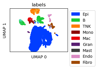
Visualize scRNA-seq data¶

Create UMAPs for the scRNA-seq data

[4]:

ref_umap = tc.utils.umap_single_cell_data(reference)
fig = tc.pl.scatter(ref_umap, keys='labels', position_key='X_umap', colors=labels_colors, joint=True, point_size=5, axsize=axsize, noticks=True,
axes_labels=['UMAP 0','UMAP 1']);

SCumap...SCprep...time 7.727412223815918
time 68.7538959980011

../_images/notebooks_slideseq_mouse_colon_7_1.png

Annotate the spatial data with compositions of cell types¶

Annotation is done on cell type level with multi_center=10 to capture variation within a cell type

[5]:

tc.tl.annotate(puck,reference,'labels',result_key='labels',multi_center=10,);

Starting preprocessing
Annotation profiles were not found in `reference.varm["labels"]`. Constructing reference profiles with `tacco.preprocessing.construct_reference_profiles` and default arguments...
Finished preprocessing in 14.11 seconds.
Starting annotation of data with shape (33673, 16879) and a reference of shape (17512, 16879) using the following wrapped method:
+- platform normalization: platform_iterations=0, gene_keys=labels, normalize_to=adata
   +- multi center: multi_center=10 multi_center_amplitudes=True
      +- bisection boost: bisections=4, bisection_divisor=3
         +- core: method=OT annotation_prior=None
mean,std( rescaling(gene) )  0.7410490029315331 10.559549576241444
bisection run on 1
bisection run on 0.6666666666666667
bisection run on 0.4444444444444444
bisection run on 0.2962962962962963
bisection run on 0.19753086419753085
bisection run on 0.09876543209876543
Finished annotation in 23.6 seconds.

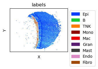
Visualize the spatial cell type distribution¶

[6]:

puck = puck[tc.sum(puck.X,axis=1)>=50].copy() # restrict downstream analysis to "good" beads
fig = tc.pl.scatter(puck, keys='labels', position_key=['x','y'], colors=labels_colors, joint=True, point_size=1, axsize=axsize, noticks=True, axes_labels=['X','Y']);

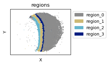
../_images/notebooks_slideseq_mouse_colon_11_0.png

Find spatially contiguous regions of comparable expression patterns¶

[7]:

tc.tl.find_regions(puck,key_added='regions',position_weight=1, resolution=0.55);
puck.obs['regions'] = puck.obs['regions'].map(lambda x: f'region_{x}').astype('category')

WARNING: You’re trying to run this on 20388 dimensions of `.X`, if you really want this, set `use_rep='X'`.
         Falling back to preprocessing with `sc.pp.pca` and default params.

[8]:

# ensure that the region naming is deterministic
ordered_regions = puck.obs.groupby('regions')['x'].mean().sort_values()
puck.obs['regions'] = puck.obs['regions'].map({r0:r1 for r0,r1 in zip(ordered_regions.index,['region_2','region_1','region_3','region_0'])}).astype(pd.CategoricalDtype(['region_0','region_1','region_2','region_3'],ordered=True))

[9]:

fig = tc.pl.scatter(puck,'regions',joint=True,axsize=axsize, point_size=1, noticks=True, axes_labels=['X','Y'], colors=region_colors);

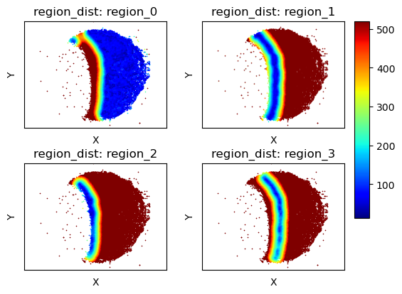
../_images/notebooks_slideseq_mouse_colon_15_0.png

Get regularized distances from these regions¶

[10]:

tc.tl.annotation_coordinate(puck,annotation_key='regions',result_key='region_dist',max_distance=500,delta_distance=20,sparse=False);

annotation_distance: The argument `distance_key` is `None`, meaning that the distance which is now calculated on the fly will not be saved. Providing a precalculated distance saves time in multiple calls to this function.
calculating distance for sample 1/1

[11]:

fig,axs=tc.pl.subplots(2,2,axsize=axsize,x_padding=0.5,y_padding=0.5)
axs=axs.flatten()[:,None]
fig = tc.pl.scatter(puck,'region_dist',cmap='jet', joint=False,axsize=axsize, point_size=1, noticks=True, axes_labels=['X','Y'], ax=axs);
for i in [-4,-2,-1]:
    fig.axes[i].remove()

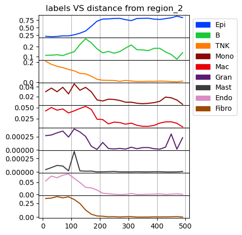
../_images/notebooks_slideseq_mouse_colon_18_0.png

Cell type composition at a certain regularized distance

[12]:

fig = tc.pl.annotation_coordinate(puck,annotation_key='labels',coordinate_key=('region_dist','region_2'),colors=labels_colors,max_coordinate=500,delta_coordinate=20, axsize=(3,0.45));

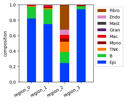
../_images/notebooks_slideseq_mouse_colon_20_0.png

Cell type composition in the regions¶

[13]:

fig = tc.pl.compositions(puck, 'labels', 'regions', colors=labels_colors, axsize=(2.4,2.5));

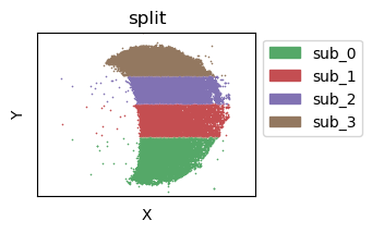
../_images/notebooks_slideseq_mouse_colon_22_0.png

Subdivide the single spatial sample spatially into several parts¶

[14]:

tc.utils.spatial_split(puck, position_key='y', position_split=4, result_key='split');
puck.obs['split'] = split_names[puck.obs['split'].astype('category').cat.codes]
puck.obs['split'] = puck.obs['split'].astype('category')
fig = tc.pl.scatter(puck, 'split', joint=True,axsize=axsize, point_size=1, noticks=True, axes_labels=['X','Y'], colors=split_colors);

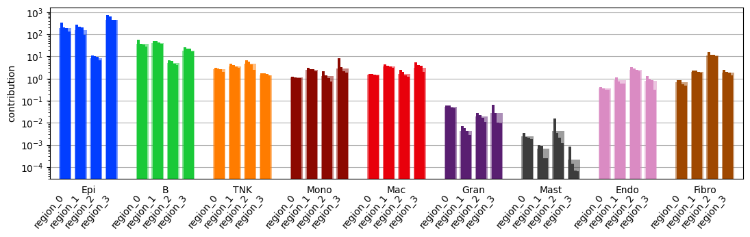
../_images/notebooks_slideseq_mouse_colon_24_0.png

Compare cell type composition across these parts

[15]:

fig = tc.pl.contribution(puck, 'labels', 'regions', colors=labels_colors, normalization='gmean', reduction='sum', sample_key='split', axsize=(len(puck.obsm['labels'].columns) * (0.2 * 4 + .1) * 1.25, 2.5));

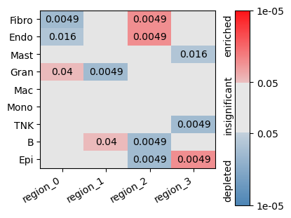
../_images/notebooks_slideseq_mouse_colon_26_0.png

Do statistics on these parts treating them as independent samples

[16]:

enr = tc.tl.enrichments(puck, 'labels', 'regions', normalization='gmean', reduction='sum', sample_key='split');
fig = tc.pl.significances(enr, p_key='p_mwu_fdr_bh', value_key='labels', group_key='regions', axsize=(2.5,len(puck.obsm['labels'].columns)*0.25));

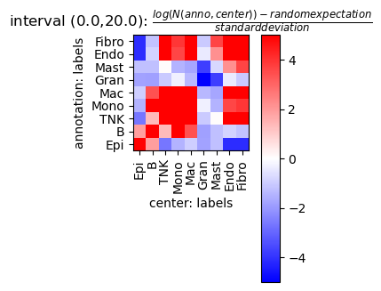
../_images/notebooks_slideseq_mouse_colon_28_0.png

Analyse neighbourhips¶

[17]:

tc.tl.co_occurrence_matrix(puck,annotation_key='labels',result_key='labels-labels',max_distance=20,n_permutation=10, );
fig = tc.pl.co_occurrence_matrix(puck,analysis_key='labels-labels',score_key='z',cmap_vmin_vmax=(-5,5), axsize=(1.3,1.3));

co_occurrence: The argument `distance_key` is `None`, meaning that the distance which is now calculated on the fly will not be saved. Providing a precalculated distance saves time in multiple calls to this function.
calculating distance for sample 1/1
The heuristic value for the parameter `numba_blocksize` is 160.0. Consider specifying this directly as argument to avoid (possibly significant) overhead and/or experiment with this value on (a subset of) the actual dataset at hand to obtain an optimal value in terms of speed and memory requirements.

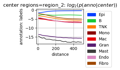
../_images/notebooks_slideseq_mouse_colon_30_1.png

Analyse cell type composition relative to a region annotation¶

Calculate cell type composition in dependence of the distance to region_2. In contrast to the analysis above using a gobally defined regularized distance, the distance here is defined for all pairs of observations and aggregated over the pairs.

[18]:

tc.tl.co_occurrence(puck,annotation_key='labels',center_key='regions',result_key='labels-regions',delta_distance=20,max_distance=500,n_permutation=10, );
fig = tc.pl.co_occurrence(puck,analysis_key='labels-regions',score_key='log_composition',colors=labels_colors, log_base=2, show_only_center=['region_2'], axsize=np.array([4,3])*0.4);

co_occurrence: The argument `distance_key` is `None`, meaning that the distance which is now calculated on the fly will not be saved. Providing a precalculated distance saves time in multiple calls to this function.
calculating distance for sample 1/1
The heuristic value for the parameter `numba_blocksize` is 500.0. Consider specifying this directly as argument to avoid (possibly significant) overhead and/or experiment with this value on (a subset of) the actual dataset at hand to obtain an optimal value in terms of speed and memory requirements.

../_images/notebooks_slideseq_mouse_colon_32_1.png