Co-occurrence computations

This example demonstrates co-occurrence analyses with TACCO using mouse olfactory bulb Slide-Seq (Wang et al.) and scRNA-seq data (Tepe et al.). It also sompares co-occurence related analyses with the Squidpy implementation (Palla et al.).

(Wang et al.): Wang IH, Murray E, Andrews G, Jiang HC et al. Spatial transcriptomic reconstruction of the mouse olfactory glomerular map suggests principles of odor processing. Nat Neurosci 2022 Apr;25(4):484-492. PMID: 35314823

(Tepe et al.): Tepe B, Hill MC, Pekarek BT, Hunt PJ et al. Single-Cell RNA-Seq of Mouse Olfactory Bulb Reveals Cellular Heterogeneity and Activity-Dependent Molecular Census of Adult-Born Neurons. Cell Rep 2018 Dec 4;25(10):2689-2703.e3. PMID: 30517858

(Palla et al.): Palla, G., Spitzer, H., Klein, M. et al. Squidpy: a scalable framework for spatial omics analysis. Nat Methods 19, 171–178 (2022). https://doi.org/10.1038/s41592-021-01358-2

import os
import sys
import matplotlib
import time

import pandas as pd
import numpy as np
import anndata as ad

import tacco as tc
import squidpy as sq

# The notebook expects to be executed either in the workflow directory or in the repository root folder...
sys.path.insert(1, os.path.abspath('workflow' if os.path.exists('workflow/common_code.py') else '..'))
import common_code

Load data

data_path = common_code.find_path('results/slideseq_mouse_olfactory_bulb')
plot_path = common_code.find_path('results/cooccurrence',create_if_not_existent=True)

reference = ad.read(f'{data_path}/reference.h5ad')

pucks = ad.concat({ key: ad.read(f'{data_path}/{key}.h5ad') for key in ['puck_1_4','puck_1_5','puck_1_6','puck_1_7',] }, label='puck', index_unique='-')

Annotate the spatial data with compositions of cell types

Annotation is done with multi_center=10 to capture within type heterogeneity

tc.tl.annotate(pucks,reference,'type',result_key='type',multi_center=10,verbose=0);

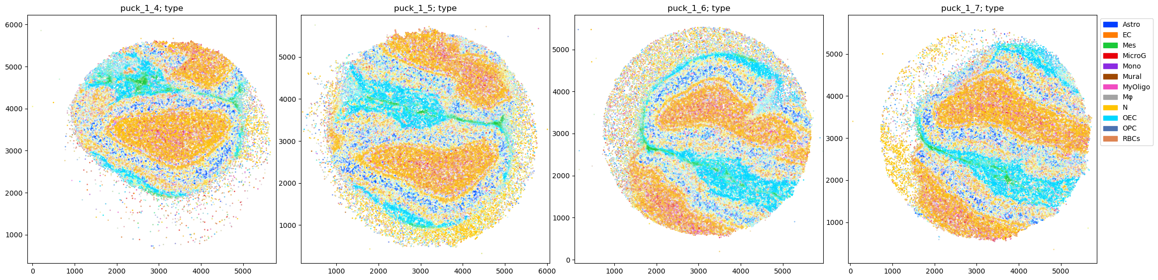
fig = tc.pl.scatter(pucks, 'type', group_key='puck');

Full cell type names

reference.obs[['type','long']].drop_duplicates().reset_index(drop=True)

	type	long
0	OEC	olfactory ensheathing cell-based (Sox10+)
1	Astro	astrocytic (Gfap+)
2	N	neuronal (Syt1+/Tubb3+)
3	EC	endothelial (Slco1c1+)
4	MicroG	microglia (Aif1+/Siglech+)
5	MyOligo	myelinating-oligodendrocyte-based (Mag+)
6	Mes	mesenchymal
7	Mφ	macrophage (Aif1+/Cd52+)
8	OPC	oligodendrocyte-precursor-based (Olig2+)
9	Mono	monocyte (Aif1+/Cd74+)
10	Mural	mural (Pdgfrb+)
11	RBCs	red blood cell (Aif1+/Hba-a1+)

Co-occurrence calculation for a single spatial sample and one annotation

Spatial analyses assume that there is a well defined distance between all observations. That is only the case for a single spatial sample (see below for the analysis of multiple samples together). So we start by demonstrating the various flavours of co-occurrence related analyses implemented in TACCO on a single Slide-seq sample.

single_puck = pucks.query('puck=="puck_1_5"').copy()

Prepare distance-based analyses

In TACCO, most spatial analyses are based on the same core functionality: calculating a distance matrix between observations and generating statistics about the co-occurrence of annotations of these observations. Therefore the “heavy lifting” is done only once in a call to tc.tl.co_occurrence.

As the spatial analyses bin the neighbourship relations in bins of finite width, it makes sense to specify this explicitly to have a well defined and biologically meaningful bin size: delta_distance=20, in units of the positional annotation, here in µm.

As the samples have a finite spatial size it further makes sense to specify a maximum size to look at which is much smaller than the spatial sample size (to remove boundary artefacts) but still contains all interesting biology: max_distance=1000, here also in µm.

TACCO can compute dense and sparse distance matrices. Using sparse matrices is necessary for very large datasets and then reduces the computational and memory load drastically. But for “small” samples with a couple 10k observations, using dense distance matrices is actually faster as dense matrix operations are intrinsically faster, which outweighs the performance gain of the sparse calculation in these cases. So we use a dense distance calculation here: sparse=False.

tc.tl.co_occurrence(single_puck, 'type', result_key='type-type', delta_distance=20, max_distance=1000, sparse=False);

co_occurrence: The argument `distance_key` is `None`, meaning that the distance which is now calculated on the fly will not be saved. Providing a precalculated distance saves time in multiple calls to this function.
calculating distance for sample 1/1

Flavors of spatial relationships

Composition

The most basic observables are the counts of observations of annotation-pairs per distance bin. For non-categorical annotations the values in the .obs matrix are used to update all annotaion-pairs simultaneously instead of putting a 1 for the single occurring annotation-pair.

If these counts are normalized for a “center” annotation per distance bin, we get a rather simple quantity, which we call “composition”. We can plot this as a function of distance.

We can directly see some strong features in the data, e.g. that the direct neighbourhoods (distance <50µm) of Mesenchymal cells (Mes) consist of much more Mesenchymal cells than further away (distance >300µm), which could be indicative of a spatially localized enrichment of Mesenchymal cells. And indeed comparing to the scatter plot above, we see that these cells indeed appear localized in the thin midplane separating the two halves of the olfactory bulb.

But aside from that we mainly see a global ladder of cell type frequency, which only reflects the pseodo-bulk cell type fractions, e.g. that Neurons (N) are the most frequent neighbours of (nearly) all cell types at (nearly) all distances.

On the log scale we can also see some similar local enrichment features as for the Mesenchymal cells also for the myelinating oligodendrocyte-based cells (MyOligo) and red blood cells (RBC). They appear on a much lower scale, as the base frequency of these cell types is just much lower.

fig = tc.pl.co_occurrence(single_puck, 'type-type', score_key='composition', wspace=0.25);

fig = tc.pl.co_occurrence(single_puck, 'type-type', score_key='log_composition', log_base=2, wspace=0.25);

Co-occurrence

As the information accessible in the “composition” view is dominated by the overall cell type fractions, it would be nice to factor them out.

That is exactly what the “co-occurrence” does: it normalizes the “composition” by an additional factor of overall cell type frequency. It is a measure for overrepresentation of a cell type at a certain distance of some center cell type compared to the overall cell type frequency.

As this divides out uninteresting global information, the remaining information can be displayed in a much clearer way. E.g. everything happens on the same scale.

If we assume that for very long distances there is no correlation between the annotation of observations, then the “co-occurrence” converges to a value of 1, as the cell type frequency in the neighbourship at large distances exactly equals the overall cell type fractions. In the displayed sample thiss happens at the latest around 1000µm, which is the reason to use this value as maximum distance.

While this puts the relevant features on the same scale already, using a logarithmic representation can still be helpful, as it symmetrizes the dynamic range of fold changes: the bare “co-occurrence” has a dynamic range for underrepresentation from 0 to 1 and for overrepresentation from 1 to infinity, while the loarithmized quantity goes from -infinity to 0 for underrepresentation and from 0 to infinity for overrepresentation. On the log scale, the quantity approaches 0 for large distances.

The “co-occurrence” makes many more subtle features of distance dependent over- and underrepresentation visible. Here we can see a lot of general features in the spatial beaviour of spatial data. There are generally short distance features covering distances up to a couple of cell-sizes which represent local correlations and interactions between the cell types. They are visible on top of a long range background which decays to the long-distance 0 (or 1) and predominantely describes the large scale tissue structure for structured samples.

fig = tc.pl.co_occurrence(single_puck, 'type-type', score_key='occ', wspace=0.25);

fig = tc.pl.co_occurrence(single_puck, 'type-type', score_key='log_occ', log_base=2, wspace=0.25);

Distance distribution

The distance dependent “composition” and its relative version the “co-occurrence” are just two examples of quantities which one can look at in this context. An in some sense orthogonal approach is to normalize the annotation pair counts not per distance bin, but instead across distance bins separately for each annotation pair, we get a quantity which can be interpreted as a distribution of neighbourship counts across distances, which we call “distance distribution”.

Unlike the “composition”, the “distance distribution” is not dominated by the overall cell type distribution, but instead by the overall spatial distribution of cell types, which can be approximated locally for small distances by a uniform distribution. This is seen as the linear dependence for small distances: If the distance doubles, there is twice the amount of neighbourship relations per distance bin, as the circumference of a circle is just proportional to its radius. As the sample is of finite size, we also see a generic bending down of the distributions which leads to another intersection with 0 at the largest distance in the sample. This effect can mostly be ignored if we restrict our attention to distances much smaller than the sample size.

Here we need to get rid of this dominating geometric behaviour, and this time a log does not help at all.

What we see nevertheless, are again very strong features: The deviation of the linear behaviour for small distances indicates the deviation of the uniform distribution of a certain cell type around a center cell type, which is again clearly visible for the neighbourship relations of the Mesenchymal cells.

fig = tc.pl.co_occurrence(single_puck, 'type-type', score_key='distance_distribution', wspace=0.25);

fig = tc.pl.co_occurrence(single_puck, 'type-type', score_key='log_distance_distribution', log_base=2, wspace=0.25);

Relative distance distribution

Instead of analytically remove the expected features from the data, we can again normalize it out if we consider the “distance distribution” of a certain cell type relative to the “distance distribution” of all observations ignoring the cell type. We call this the “relative distance distribution”.

While constructed in a completely different way, the features appearing in this quantity are very similar to the ones seen in the “co-occurrence”.

There is one important difference: The “relative distance distribution” is harder to interpret the long range behaviour enters the values of short range quantities via the normalization across all distances. The distribution itself must sum to 1, so whenever we have a deviation in the ratio at short distances, it must be compensated at longer distances. This leads to an earlier appearance of the values 1 and 0 at finite distances rather than being the limiting behaviour for large distances as is the case for the “co-occurrence”. While this can be used to define an interaction length scale for each cell type pair (or approximately for each center cell type), it makes the interpretation of these plots harder, so the “co-occurrence” is prefered in practive. Still it is helps to understand the generic properties of spatial data.

fig = tc.pl.co_occurrence(single_puck, 'type-type', score_key='relative_distance_distribution', wspace=0.25);

fig = tc.pl.co_occurrence(single_puck, 'type-type', score_key='log_relative_distance_distribution', log_base=2, wspace=0.25);

Co-occurrence calculation for a single spatial sample and two different annotations

Sometimes one is not just interested in the spatial relations of an annotation with itself, e.g. of one cell type with another cell type, but between two annotations, e.g. cell type and tissue annotations or expression programs.

As an example, we generate a second ad-hoc annotation for this dataset, which is based on some selected marker genes. They do not carry information orthogonal to the cell types, but can illustrate the use case.

We still work with a single puck.

pucks.obsm['marker'] = pd.DataFrame(index=pucks.obs.index)
for marker in ['Cd68','Cd4','Cd8a','Epcam','Vwf','Rbfox3']:
    pucks.obsm['marker'][marker] = tc.sum(pucks[:,[marker]].X,axis=1)
pucks.obsm['marker']['other'] = tc.sum(pucks.X,axis=1) - tc.sum(pucks.obsm['marker'],axis=1)
pucks.obsm['marker'] /= tc.sum(pucks.obsm['marker'],axis=1).to_numpy()[:,None]

single_puck = pucks.query('puck=="puck_1_5"').copy()

Prepare distance-based analyses

As we have have now two (compositional) annotations “type” and “marker”, we can create four sets of co-occurrence annotation pairs: “type-type”,”marker-type”,”type-marker”, and “marker-marker”. For this we need to run tc.tl.co_occurrence four times.

Note that we can calculate the distance only once and supply it to the successive calls of the function (this is actually what the message was telling us all along). We do this here for demonstation purposes, but it is not really necessary: distance calculation is fast enough for interactively working with this data set.

%time tc.tl.distance_matrix(single_puck, max_distance=np.inf, result_key='precomputed');

CPU times: user 7.67 s, sys: 11.8 s, total: 19.5 s
Wall time: 2.77 s

AnnData object with n_obs × n_vars = 44311 × 19742
    obs: 'x', 'y', 'puck'
    uns: 'type_mc10'
    obsm: 'type_mc10', 'type', 'marker'
    varm: 'type_mc10'
    obsp: 'precomputed'

tc.tl.co_occurrence(single_puck, 'type', center_key='type', result_key='type-type', delta_distance=20, max_distance=1000, distance_key='precomputed');
tc.tl.co_occurrence(single_puck, 'marker', center_key='type', result_key='marker-type', delta_distance=20, max_distance=1000, distance_key='precomputed');
tc.tl.co_occurrence(single_puck, 'type', center_key='marker', result_key='type-marker', delta_distance=20, max_distance=1000, distance_key='precomputed');
tc.tl.co_occurrence(single_puck, 'marker', center_key='marker', result_key='marker-marker', delta_distance=20, max_distance=1000, distance_key='precomputed');

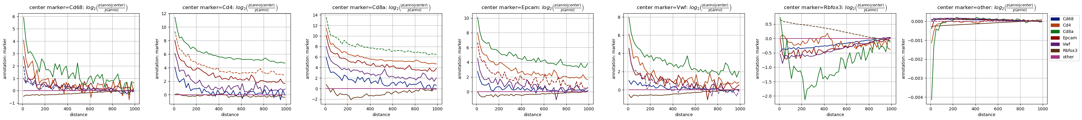
Co-occurrence

As the most straightforward spatial observable we focus here on the co-occurrence and plot it for the four cases. To not confuse the cell type and marker annotation with each other, we chose a set of different colors for the markers.

The two mixed cases ‘marker-type’ and ‘type-marker’ are not symmetric, as they are normalized (and then also plotted) differently and carry different information.

The most obvious feature of the plots involving the ‘marker’ annotation is that they look much more noisy than the ones with cell types: The reason is quite simple: the marker “signatures” are based on single genes only, which are far less covered than the cell types “signatures” which are based on information from the full transcriptome.

Despite the apparent noise we can see some features in the plots: Some make a lot of sense, e.g. that the neural marker Rbfox3 (aka NeuN) behaves qualitatively similar to the neuronal cell type (N), as do Cd4/Cd68 with Monocytes (Mono) and Macrophages (Mφ).

marker_colors = tc.pl.get_default_colors(single_puck.obsm['marker'].columns, offset=20)

fig = tc.pl.co_occurrence(single_puck, 'type-type', score_key='log_occ', log_base=2, wspace=0.25);
fig = tc.pl.co_occurrence(single_puck, 'marker-type', score_key='log_occ', log_base=2, wspace=0.25, colors=marker_colors);
fig = tc.pl.co_occurrence(single_puck, 'type-marker', score_key='log_occ', log_base=2, wspace=0.25);
fig = tc.pl.co_occurrence(single_puck, 'marker-marker', score_key='log_occ', log_base=2, wspace=0.25, colors=marker_colors);

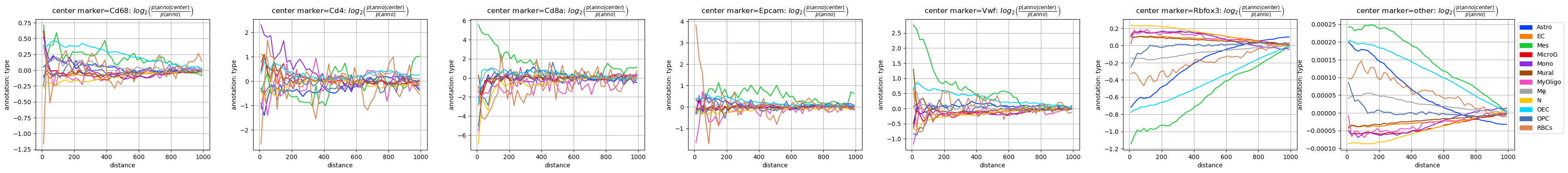
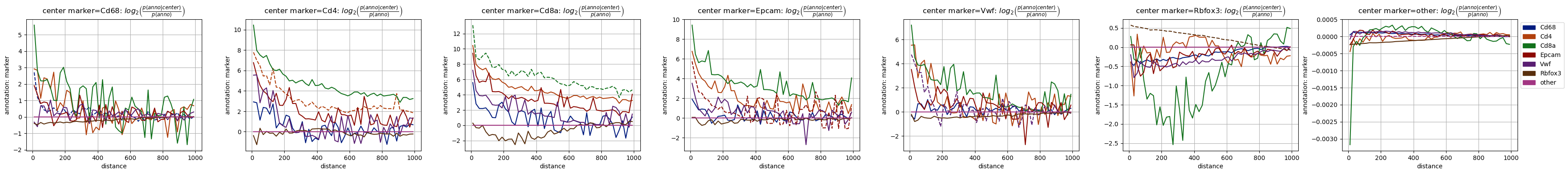
But there are also some more puzzling observations, like the very similar behaviour of the T cell marker Cd8a and mesenchymal annotation (Mes) - this is completely unexpected. Luckily, we can quickly check the data to see where this finding comes from.

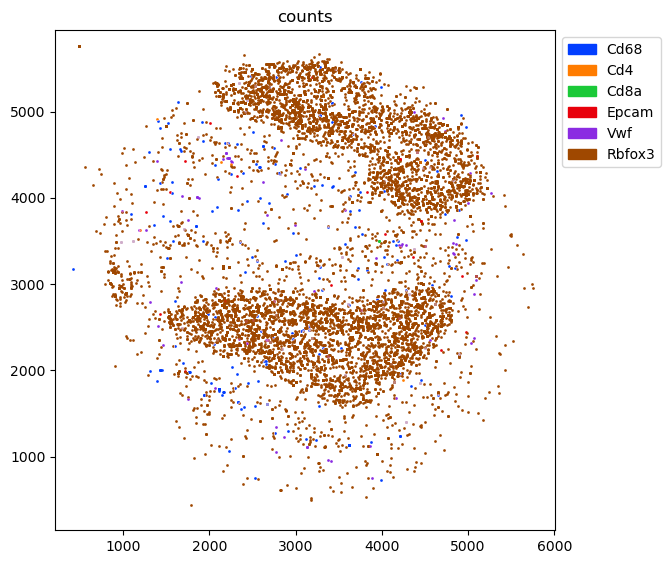
We start by looking at the spatial distribution of the counts of the marker genes. There we can hardly find any Cd8a expression. So maybe it is very lowly covered/expressed and just happens to be close to Mesenchymal annotation? After all, there was not even a single T cell in the single cell reference dataset.

We can check this by examining the overall expression in the sample and the number of spatial observations which expres a given marker at all. And in fact there is only a single bead with only two measured Cd8a transcripts. And this single bead was annotated with a high Mesenchymal contribution. So we can safely discard this finding - at least until we have more data: We could speculate that the few T cells which are in the mouse olfactory bulb are indeed localized in the same region as mesenchymal cells are.

single_puck.obsm['counts'] = single_puck[:,['Cd68','Cd4','Cd8a','Epcam','Vwf','Rbfox3']].to_df()
fig = tc.pl.scatter(single_puck, 'counts');

pd.DataFrame({'total_counts':single_puck.obsm['counts'].sum(axis=0),'positive_beads':(single_puck.obsm['counts']!=0).sum(axis=0),})

	total_counts	positive_beads
Cd68	222	205
Cd4	8	7
Cd8a	2	1
Epcam	21	19
Vwf	76	71
Rbfox3	7587	5277

single_puck.obsm['type'][single_puck.obsm['counts']['Cd8a']!=0]

type	Astro	EC	Mes	MicroG	Mono	Mural	MyOligo	Mφ	N	OEC	OPC	RBCs
barcodes
TCAAATGTCCGCAG-puck_1_5	0.000325	0.003029	0.834439	0.000257	0.000088	0.008671	0.000004	0.000276	0.000003	0.152907	0.000001	4.226232e-07

Co-occurrence calculation for multiple spatial samples

Separate analysis per sample

Speaking of more data, lets now see how we can incorporate multiple samples in this analysis.

As stated earlier, we cannot just concatenate all the data and treat all the samples as a single sample: the spatial distances would be calculated assuming that the coordinates mean the same thing across samples.

The first thing to try is to split the data by sample and run the analysis separately. And there is not much else we can do: It is just not possible in general to define a spatial distance between samples, so no spatial binning is possible and neither is all the analysis which builds on it. (There is always an exception to this rule, e.g. perfectly aligned consecutive sections - and this can in fact be handled by concatenating all the data and adding a z coordinate according to the stacking direction.)

We see quite a similar behaviour of the co-occurrence in different samples, so that is reassuring: These are consecutive sections from the olfactory bulb of the same mouse, so they should exhibit very similar features.

individual_pucks = {}
for puck_name,df in pucks.obs.groupby('puck'):
    individual_pucks[puck_name] = pucks[df.index].copy()
    tc.tl.co_occurrence(individual_pucks[puck_name], 'type', result_key='type-type',delta_distance=20,max_distance=1000,sparse=False,);

co_occurrence: The argument `distance_key` is `None`, meaning that the distance which is now calculated on the fly will not be saved. Providing a precalculated distance saves time in multiple calls to this function.
calculating distance for sample 1/1
co_occurrence: The argument `distance_key` is `None`, meaning that the distance which is now calculated on the fly will not be saved. Providing a precalculated distance saves time in multiple calls to this function.
calculating distance for sample 1/1
co_occurrence: The argument `distance_key` is `None`, meaning that the distance which is now calculated on the fly will not be saved. Providing a precalculated distance saves time in multiple calls to this function.
calculating distance for sample 1/1
co_occurrence: The argument `distance_key` is `None`, meaning that the distance which is now calculated on the fly will not be saved. Providing a precalculated distance saves time in multiple calls to this function.
calculating distance for sample 1/1

fig = tc.pl.co_occurrence(individual_pucks, 'type-type', wspace=0.25);

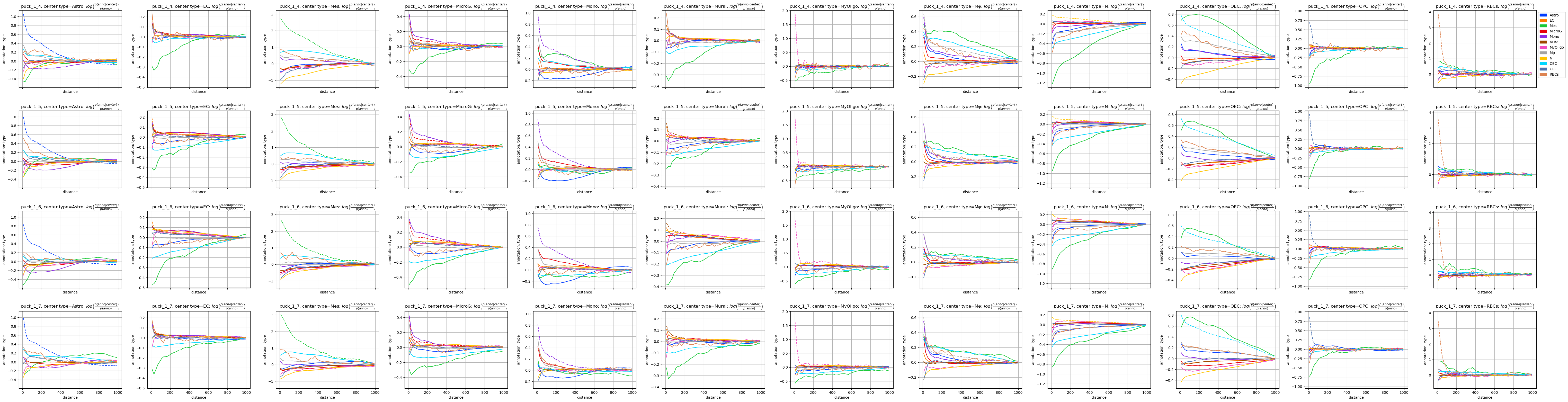
Plotting all the different samples in different rows is ok for a first glimpse at the data in a tutorial, but it is rather bulky for getting an overview over the variability. And of course we can just plot all the samples in a single row and investigate the variability across samples.

It looks like we mostly have the same signal across all pucks enriched with technical differences across the pucks.

fig = tc.pl.co_occurrence(individual_pucks, 'type-type', wspace=0.25, merged=True);

Aggregating the analysis across sample

One can reduce statistical and technical variability by simply averaging across replicates. And this is what tc.tl.co_occurrence doesautomatically if we tell it that there are multiple samples in the dataset.

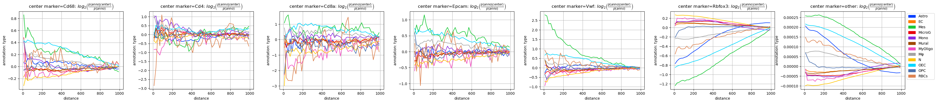
And indeed, already with four pucks instead of one and five instead of one Cd8a-positive beads, the spurious Cd8a-Mesenchymal association collapses drastically. Compared to the cell type annotation the picture is still very noisy, basically for all selected genes except for the very well covered neural marker.

An important message from this analysis is that only the statistical error can be seen in the “noisy-ness” of the curves, while the systematic error is invisible!

tc.tl.co_occurrence(pucks, 'type', center_key='type', sample_key='puck', result_key='type-type', delta_distance=20, max_distance=1000, sparse=False);
tc.tl.co_occurrence(pucks, 'marker', center_key='type', sample_key='puck', result_key='marker-type', delta_distance=20, max_distance=1000, sparse=False);
tc.tl.co_occurrence(pucks, 'type', center_key='marker', sample_key='puck', result_key='type-marker', delta_distance=20, max_distance=1000, sparse=False);
tc.tl.co_occurrence(pucks, 'marker', center_key='marker', sample_key='puck', result_key='marker-marker', delta_distance=20, max_distance=1000, sparse=False);

co_occurrence: The argument `distance_key` is `None`, meaning that the distance which is now calculated on the fly will not be saved. Providing a precalculated distance saves time in multiple calls to this function.
calculating distance for sample 1/4
calculating distance for sample 2/4
calculating distance for sample 3/4
calculating distance for sample 4/4
co_occurrence: The argument `distance_key` is `None`, meaning that the distance which is now calculated on the fly will not be saved. Providing a precalculated distance saves time in multiple calls to this function.
calculating distance for sample 1/4
calculating distance for sample 2/4
calculating distance for sample 3/4
calculating distance for sample 4/4
co_occurrence: The argument `distance_key` is `None`, meaning that the distance which is now calculated on the fly will not be saved. Providing a precalculated distance saves time in multiple calls to this function.
calculating distance for sample 1/4
calculating distance for sample 2/4
calculating distance for sample 3/4
calculating distance for sample 4/4
co_occurrence: The argument `distance_key` is `None`, meaning that the distance which is now calculated on the fly will not be saved. Providing a precalculated distance saves time in multiple calls to this function.
calculating distance for sample 1/4
calculating distance for sample 2/4
calculating distance for sample 3/4
calculating distance for sample 4/4

fig = tc.pl.co_occurrence(pucks, 'type-type', score_key='log_occ', log_base=2, wspace=0.25);
fig = tc.pl.co_occurrence(pucks, 'marker-type', score_key='log_occ', log_base=2, wspace=0.25, colors=marker_colors);
fig = tc.pl.co_occurrence(pucks, 'type-marker', score_key='log_occ', log_base=2, wspace=0.25);
fig = tc.pl.co_occurrence(pucks, 'marker-marker', score_key='log_occ', log_base=2, wspace=0.25, colors=marker_colors);

pucks.obsm['counts'] = pucks[:,['Cd68','Cd4','Cd8a','Epcam','Vwf','Rbfox3']].to_df()
pd.DataFrame({('single_puck','total_counts'):single_puck.obsm['counts'].sum(axis=0),('single_puck','positive_beads'):(single_puck.obsm['counts']!=0).sum(axis=0),('four_pucks','total_counts'):pucks.obsm['counts'].sum(axis=0),('four_pucks','positive_beads'):(pucks.obsm['counts']!=0).sum(axis=0),})

	single_puck		four_pucks
	total_counts	positive_beads	total_counts	positive_beads
Cd68	222	205	801	725
Cd4	8	7	22	19
Cd8a	2	1	6	5
Epcam	21	19	56	53
Vwf	76	71	206	193
Rbfox3	7587	5277	28259	19188

Compare TACCOs co-occurrence analysis with the one from Squidpy

Use categorically annotated data delivered with Squidpy, as Squidpy does not support this type of analysis with compositional annnotation

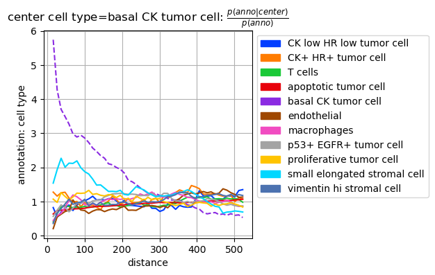
Cooccurrence analysis with Squidpy

adata_squidpy = sq.datasets.imc()
sq.gr.co_occurrence(adata_squidpy, cluster_key="cell type")
sq.pl.co_occurrence(adata_squidpy, cluster_key="cell type", clusters="basal CK tumor cell", figsize=(6,4))

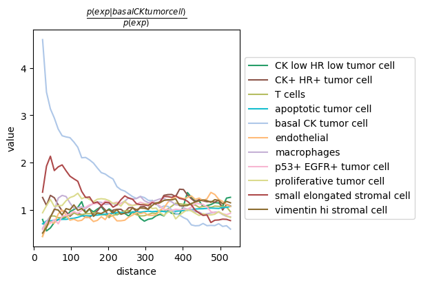
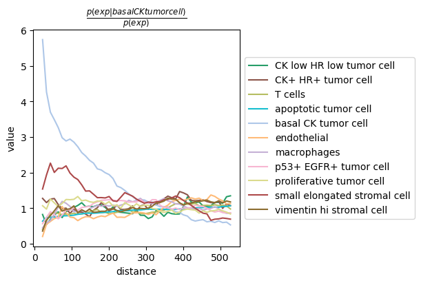
Co-occurrence analysis with TACCO

We adjust the parameters to match the Squidpy result as closely as possible

max_dist = adata_squidpy.uns[f'cell type_co_occurrence']['interval'][-1]
adata_tacco = sq.datasets.imc()
tc.tl.co_occurrence(adata_tacco, annotation_key="cell type", position_key='spatial', result_key=f'cell type_co_occurrence', max_distance=max_dist, sparse=False, delta_distance=max_dist/50)
tc.pl.co_occurrence(adata_tacco, analysis_key=f'cell type_co_occurrence', score_key='occ', show_only_center="basal CK tumor cell", axsize=(3,3));

co_occurrence: The argument `distance_key` is `None`, meaning that the distance which is now calculated on the fly will not be saved. Providing a precalculated distance saves time in multiple calls to this function.
calculating distance for sample 1/1

Result format is Squidpy compatible so that the Tacco result can be plotted with Squidpy.

sq.pl.co_occurrence(adata_tacco, cluster_key="cell type", clusters="basal CK tumor cell", figsize=(6,4))

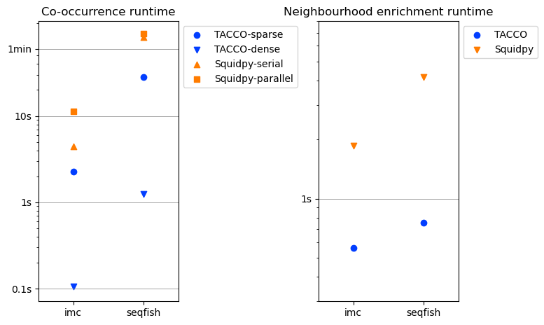
Compare timing for co-occurrences

def time_co_occurrence(label, adata, annotation_key):
    # measure always the second execution to avoid overhead from jitting etc.
    timings = []

    sq.gr.co_occurrence(adata, cluster_key=annotation_key, n_jobs=tc.utils.cpu_count())
    start = time.time()
    sq.gr.co_occurrence(adata, cluster_key=annotation_key, n_jobs=tc.utils.cpu_count())
    end = time.time()
    timings.append((label,'Squidpy-parallel',end-start))

    sq.gr.co_occurrence(adata, cluster_key=annotation_key)
    start = time.time()
    sq.gr.co_occurrence(adata, cluster_key=annotation_key)
    end = time.time()
    timings.append((label,'Squidpy-serial',end-start))

    max_dist = adata.uns[f'{annotation_key}_co_occurrence']['interval'][-1]

    tc.tl.co_occurrence(adata, annotation_key=annotation_key, position_key='spatial', result_key=f'{annotation_key}_co_occurrence', max_distance=max_dist, sparse=False, delta_distance=max_dist/50);
    start = time.time()
    tc.tl.co_occurrence(adata, annotation_key=annotation_key, position_key='spatial', result_key=f'{annotation_key}_co_occurrence', max_distance=max_dist, sparse=False, delta_distance=max_dist/50);
    end = time.time()
    timings.append((label,'TACCO-dense',end-start))

    tc.tl.co_occurrence(adata, annotation_key=annotation_key, position_key='spatial', result_key=f'{annotation_key}_co_occurrence', max_distance=max_dist, sparse=True, delta_distance=max_dist/50);
    start = time.time()
    tc.tl.co_occurrence(adata, annotation_key=annotation_key, position_key='spatial', result_key=f'{annotation_key}_co_occurrence', max_distance=max_dist, sparse=True, delta_distance=max_dist/50);
    end = time.time()
    timings.append((label,'TACCO-sparse',end-start))

    return timings

timings_cooc = []
timings_cooc.extend(time_co_occurrence('imc', sq.datasets.imc(), "cell type"))
timings_cooc.extend(time_co_occurrence('seqfish', sq.datasets.seqfish(), 'celltype_mapped_refined'))

timings_cooc = pd.DataFrame(timings_cooc,columns=['dataset','method','time (s)'])

timings_cooc['method'] = timings_cooc['method'].astype(pd.CategoricalDtype(['TACCO-sparse','TACCO-dense','Squidpy-serial','Squidpy-parallel'],ordered=True))

co_occurrence: The argument `distance_key` is `None`, meaning that the distance which is now calculated on the fly will not be saved. Providing a precalculated distance saves time in multiple calls to this function.
calculating distance for sample 1/1
co_occurrence: The argument `distance_key` is `None`, meaning that the distance which is now calculated on the fly will not be saved. Providing a precalculated distance saves time in multiple calls to this function.
calculating distance for sample 1/1
co_occurrence: The argument `distance_key` is `None`, meaning that the distance which is now calculated on the fly will not be saved. Providing a precalculated distance saves time in multiple calls to this function.
calculating distance for sample 1/1
The heuristic value for the parameter `numba_blocksize` is 530.0. Consider specifying this directly as argument to avoid (possibly significant) overhead and/or experiment with this value on (a subset of) the actual dataset at hand to obtain an optimal value in terms of speed and memory requirements.
co_occurrence: The argument `distance_key` is `None`, meaning that the distance which is now calculated on the fly will not be saved. Providing a precalculated distance saves time in multiple calls to this function.
calculating distance for sample 1/1
The heuristic value for the parameter `numba_blocksize` is 530.0. Consider specifying this directly as argument to avoid (possibly significant) overhead and/or experiment with this value on (a subset of) the actual dataset at hand to obtain an optimal value in terms of speed and memory requirements.

co_occurrence: The argument `distance_key` is `None`, meaning that the distance which is now calculated on the fly will not be saved. Providing a precalculated distance saves time in multiple calls to this function.
calculating distance for sample 1/1
co_occurrence: The argument `distance_key` is `None`, meaning that the distance which is now calculated on the fly will not be saved. Providing a precalculated distance saves time in multiple calls to this function.
calculating distance for sample 1/1
co_occurrence: The argument `distance_key` is `None`, meaning that the distance which is now calculated on the fly will not be saved. Providing a precalculated distance saves time in multiple calls to this function.
calculating distance for sample 1/1
The heuristic value for the parameter `numba_blocksize` is 3.2. Consider specifying this directly as argument to avoid (possibly significant) overhead and/or experiment with this value on (a subset of) the actual dataset at hand to obtain an optimal value in terms of speed and memory requirements.
co_occurrence: The argument `distance_key` is `None`, meaning that the distance which is now calculated on the fly will not be saved. Providing a precalculated distance saves time in multiple calls to this function.
calculating distance for sample 1/1
The heuristic value for the parameter `numba_blocksize` is 3.2. Consider specifying this directly as argument to avoid (possibly significant) overhead and/or experiment with this value on (a subset of) the actual dataset at hand to obtain an optimal value in terms of speed and memory requirements.

def time_neighbourhood_enrichment(label, adata, annotation_key):
    # measure always the second execution to avoid overhead from jitting etc.
    timings = []

    # let squidpy figure out the distance scale
    sq.gr.spatial_neighbors(adata)
    radius = adata.obsp['spatial_distances'].data.mean()

    sq.gr.spatial_neighbors(adata, coord_type='generic', radius=radius)
    sq.gr.nhood_enrichment(adata, cluster_key=annotation_key,)
    start = time.time()
    sq.gr.spatial_neighbors(adata, coord_type='generic', radius=radius)
    sq.gr.nhood_enrichment(adata, cluster_key=annotation_key,)
    end = time.time()
    timings.append((label,'Squidpy',end-start))

    tc.tl.co_occurrence_matrix(adata, annotation_key=annotation_key, position_key='spatial', result_key=f'{annotation_key}_co_occurrence', max_distance=radius, sparse=True, n_permutation=1000)
    start = time.time()
    tc.tl.co_occurrence_matrix(adata, annotation_key=annotation_key, position_key='spatial', result_key=f'{annotation_key}_co_occurrence', max_distance=radius, sparse=True, n_permutation=1000)
    end = time.time()
    timings.append((label,'TACCO',end-start))

    return timings

timings_neigh = []
timings_neigh.extend(time_neighbourhood_enrichment('imc', sq.datasets.imc(), "cell type"))
timings_neigh.extend(time_neighbourhood_enrichment('seqfish', sq.datasets.seqfish(), 'celltype_mapped_refined'))

timings_neigh = pd.DataFrame(timings_neigh,columns=['dataset','method','time (s)'])

timings_neigh['method'] = timings_neigh['method'].astype(pd.CategoricalDtype(['TACCO','Squidpy'],ordered=True))

co_occurrence: The argument `distance_key` is `None`, meaning that the distance which is now calculated on the fly will not be saved. Providing a precalculated distance saves time in multiple calls to this function.
calculating distance for sample 1/1
The heuristic value for the parameter `numba_blocksize` is 97.0. Consider specifying this directly as argument to avoid (possibly significant) overhead and/or experiment with this value on (a subset of) the actual dataset at hand to obtain an optimal value in terms of speed and memory requirements.
co_occurrence: The argument `distance_key` is `None`, meaning that the distance which is now calculated on the fly will not be saved. Providing a precalculated distance saves time in multiple calls to this function.
calculating distance for sample 1/1
The heuristic value for the parameter `numba_blocksize` is 97.0. Consider specifying this directly as argument to avoid (possibly significant) overhead and/or experiment with this value on (a subset of) the actual dataset at hand to obtain an optimal value in terms of speed and memory requirements.

co_occurrence: The argument `distance_key` is `None`, meaning that the distance which is now calculated on the fly will not be saved. Providing a precalculated distance saves time in multiple calls to this function.
calculating distance for sample 1/1
The heuristic value for the parameter `numba_blocksize` is 0.28. Consider specifying this directly as argument to avoid (possibly significant) overhead and/or experiment with this value on (a subset of) the actual dataset at hand to obtain an optimal value in terms of speed and memory requirements.
co_occurrence: The argument `distance_key` is `None`, meaning that the distance which is now calculated on the fly will not be saved. Providing a precalculated distance saves time in multiple calls to this function.
calculating distance for sample 1/1
The heuristic value for the parameter `numba_blocksize` is 0.28. Consider specifying this directly as argument to avoid (possibly significant) overhead and/or experiment with this value on (a subset of) the actual dataset at hand to obtain an optimal value in terms of speed and memory requirements.

fig,axs = tc.pl.subplots(2, axsize=(2,4), x_padding=2)

for title,timings,ax in zip(['Co-occurrence runtime','Neighbourhood enrichment runtime'],[timings_cooc,timings_neigh],axs.flatten()):
    y = timings['time (s)']

    ynew = np.array([0.1,1,10,60,600,3600,36000])
    ynew_minor = np.concatenate([np.arange(0.1,1,0.1),np.arange(1,10,1),np.arange(10,60,10),np.arange(60,600,60),np.arange(600,3600,600),np.arange(3600,36000,3600)]).flatten()
    ynewlabels = np.array(['0.1s','1s','10s','1min','10min','1h','10h'])
    ymin = y.min() * 0.5
    ymax = y.max() * 2.0
    ynewlabels = ynewlabels[(ynew > ymin) & (ynew < ymax)]
    ynew = ynew[(ynew > ymin) & (ynew < ymax)]
    ynew_minor = ynew_minor[(ynew_minor > ymin) & (ynew_minor < ymax)]
    for yn in ynew:
        ax.axhline(yn, color='gray', linewidth=0.5)

    colors = tc.pl.get_default_colors(2)
    for im,method in enumerate(timings['method'].cat.categories):
        color = colors[method.startswith('Squidpy')]
        marker = ['o','v','^','s',][im]
        sub = timings[timings['method']==method]
        ax.scatter(sub['dataset'],sub['time (s)'], label=method, marker=marker, color=color)
    ax.set_yscale('log')

    ax.set_yticks(ynew_minor,minor=True)
    ax.set_yticks(ynew)
    ax.set_yticklabels(ynewlabels)
    ax.set_yticklabels([],minor=True)

    ax.set_xlim(-0.5,len(timings['dataset'].unique()) - 0.5)

    ax.legend(bbox_to_anchor=(1, 1), loc='upper left', ncol=1)

    ax.set_title(title)