Single molecule data: osmFISH mouse somato-sensory cortex
This example uses TACCO to annotate and analyse mouse somato-sensory cortex osmFISH data (Codeluppi et al.) and compares it to the results from Baysor (Petukhov et al.) and SSAM (Park et al.).
(Codeluppi et al.): Simone Codeluppi, Lars E. Borm, Amit Zeisel, Gioele La Manno, Josina A. van Lunteren, Camilla I. Svensson & Sten Linnarsson. Spatial organization of the somatosensory cortex revealed by osmFISH. Nat Methods 15, 932–935 (2018). https://doi.org/10.1038/s41592-018-0175-z
(Petukhov et al.): Petukhov V, Xu RJ, Soldatov RA, Cadinu P, Khodosevich K, Moffitt JR & Kharchenko PV. Cell segmentation in imaging-based spatial transcriptomics. Nat Biotechnol 40, 345–354 (2022). https://doi.org/10.1038/s41587-021-01044-w
(Park et al.): Jeongbin Park, Wonyl Choi, Sebastian Tiesmeyer, Brian Long, Lars E. Borm, Emma Garren, Thuc Nghi Nguyen, Bosiljka Tasic, Simone Codeluppi, Tobias Graf, Matthias Schlesner, Oliver Stegle, Roland Eils & Naveed Ishaque. Cell segmentation-free inference of cell types from in situ transcriptomics data. Nat Commun 12, 3545 (2021). https://doi.org/10.1038/s41467-021-23807-4
[1]:
import os
import sys
import json
import matplotlib

import pandas as pd
import numpy as np
import anndata as ad
import scanpy as sc
import seaborn as sns
import sklearn.metrics

import tacco as tc

# The notebook expects to be executed either in the workflow directory or in the repository root folder...
sys.path.insert(1, os.path.abspath('workflow' if os.path.exists('workflow/common_code.py') else '..'))
import common_code
Load data
[2]:
data_path = common_code.find_path('results/osmFISH')
[3]:
reference = ad.read(f'{data_path}/data/reference.h5ad')
rna_coords = pd.read_csv(f'{data_path}/full_anno.csv.gz')
rna_coords['ClusterName'] = rna_coords['ClusterName'].fillna('')
Plotting options
[4]:
highres = False
default_dpi = 100.0
if highres:
    matplotlib.rcParams['figure.dpi'] = 648.0
    hr_ext = '_hd'
else:
    matplotlib.rcParams['figure.dpi'] = default_dpi
    hr_ext = ''

axsize = np.array([4,3])*0.5
[5]:
color_dict = {'Inhibitory CP': '#982581',
             'Inhibitory Crhbp': '#83469b',
             'Inhibitory Cnr1':'#cb467c',
             'Inhibitory IC': '#ee519f',
             'Inhibitory Kcnip2': '#9681bd',
             'Inhibitory Pthlh': '#533594',
             'Inhibitory Vip':'#765aa6',

             'Pyramidal Cpne5':'#3a449b',
             'Pyramidal L2-3': '#10b6e7',
             'Pyramidal L2-3 L5':'#1f6a89',
             'Pyramidal Kcnip2':'#6988c4',
             'Pyramidal L3-4': '#2255a6',
             'pyramidal L4': '#8ad7ef',
             'Pyramidal L5': '#18a0b5',
             'Pyramidal L6':'#1980c4',
             'Hippocampus': '#094d73',

             'Astrocyte Gfap': '#dd4827',
             'Astrocyte Mfge8': '#f5914b',

             'Oligodendrocyte Precursor cells': '#b7d541',
             'Oligodendrocyte COP': '#6dbe45',
             'Oligodendrocyte NF': '#62a64e',
             'Oligodendrocyte MF':'#2d744b',
             'Oligodendrocyte Mature': '#27562b',

             'Perivascular Macrophages':'#752b17',
             'Microglia':'#a7633e',

             'C. Plexus': '#21b284',
             'Ependymal':'#f6e10b',

             'Pericytes':'#fac696',
             'Endothelial':'#ed2426',
             'Endothelial 1':'#f05658',
             'Vascular Smooth Muscle':'#adc471',

             '': '#D3D3D3'}
Analysis options
[6]:
method_keys = ['tacco','baysor','ssam']
method_props = pd.DataFrame({
    'ClusterName': ['osmFISH-recovered cells','single molecule annotations from mapping back the published Watershed-segmentation based annotations', 'osmFISH-recovered cells',],
    'tacco': ['TACCO', 'single molecule annotations without segmentation', 'TACCO sm annotation', ],
    'baysor': ['Baysor', 'single molecule annotations without segmentation', 'Baysor sm annotation', ],
    'ssam': ['SSAM', 'single molecule annotations from mapping back pixel-based annotations', 'SSAM sm annotation', ],
}, index=['nice_name','description','title']).T
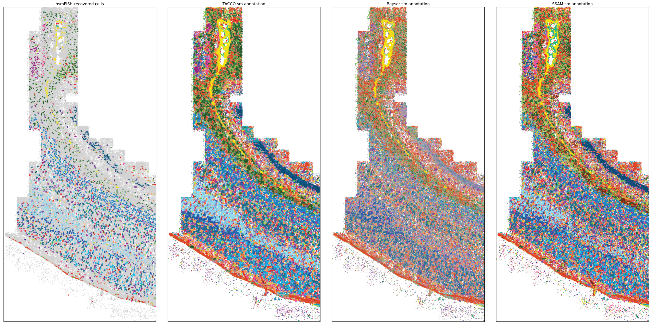
Spatial overview
Plot the single-molecule annotations for different methods to get a general overview
[7]:
fig = tc.pl.scatter(rna_coords, keys=['ClusterName', *method_keys], axsize=4e-3, joint=True, noticks=True, legend=False, colors=color_dict, point_size=1, method_labels=method_props['title']);
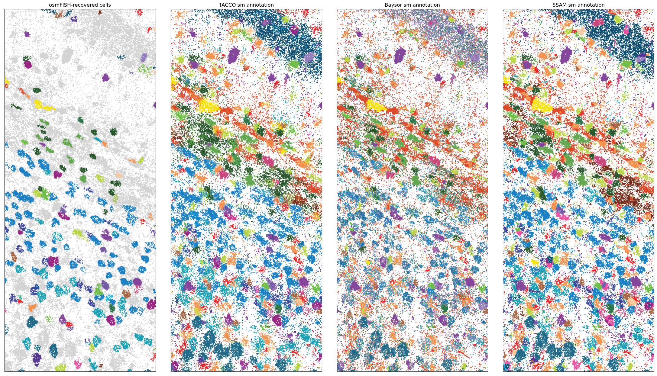
Zoom in to see the single molecules
[8]:
xmin,xmax = 1150,1400
ymin,ymax = 1000,1600 #1170,1690
query = 'x > @xmin & x < @xmax & y > @ymin & y < @ymax'

fig = tc.pl.scatter(rna_coords.query(query), keys=['ClusterName', *method_keys], axsize=2e-2, joint=True, noticks=True, legend=False, colors=color_dict, method_labels=method_props['title']);
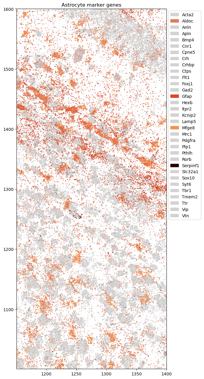
Plotting astrocyte markers
[9]:
astro_gene_colors = { 'Gfap': '#dd4827', 'Mfge8': '#f5914b', 'Aldoc': '#DE7C5A', 'Serpinf1': '#280000' }
astro_genes = list(astro_gene_colors.keys())

genes = rna_coords['gene'].unique()
gene_color_dict = {g:'#D3D3D3' for g in genes}
for g,c in astro_gene_colors.items():
    gene_color_dict[g] = c
fig = tc.pl.scatter(rna_coords.query(query), keys='gene', colors=gene_color_dict, axsize=2e-2, joint=True);
fig.get_axes()[0].set_title('Astrocyte marker genes')
[9]:
Text(0.5, 1.0, 'Astrocyte marker genes')
Analysis on the cell-like level
Process the segmented data using the recipe given in (Codeluppi et al.)
[10]:
def prep_codeluppi(adata, min_counts=0):
    adata = adata[tc.sum(adata.X,axis=1)>=min_counts]
    adata = sc.AnnData(adata.X.astype(np.float32),obs=adata.obs,var=adata.var,obsm=adata.obsm)
    sums0 = tc.sum(adata.X,axis=0)
    sums1 = tc.sum(adata.X,axis=1)
    tc.utils.col_scale(adata.X, 1/sums0)
    tc.utils.row_scale(adata.X, 1/sums1)
    adata.X *= np.prod(adata.X.shape)
    sc.tl.tsne(adata)
    return adata

def construct_segmented_data(seg_col, ann_col):
    count_data = tc.tl.dataframe2anndata(rna_coords, obs_key=seg_col, var_key='gene', compositional_keys=['ClusterName', *method_keys], mean_keys=['x','y'])
    # by construction of the TACCO segmentation, only cells composed of molecules typed with a single type are reconstructed
    # assert(((count_data.obsm[ann_col].to_numpy().flatten()==0)|(count_data.obsm[ann_col].to_numpy().flatten()==1)).all())
    # for the Baysor segmentation this is not exactly the case
    tc.utils.get_maximum_annotation(count_data, ann_col, ann_col)
    del count_data.obsm[ann_col]
    return count_data

segmented_min_counts = 20

seg_props = pd.DataFrame([
    [ 'TonT', 'TACCO segmentation\non TACCO annotation', 'tacco_seg', 'tacco', 'TACCO segmentation', 'TACCO'],
    [ 'TonB', 'TACCO segmentation\non Baysor annotation', 'baysor_seg', 'baysor', 'TACCO segmentation', 'Baysor'],
    [ 'TonS', 'TACCO segmentation\non SSAM annotation', 'ssam_seg', 'ssam', 'TACCO segmentation', 'SSAM'],
    [ 'BonB', 'Baysor segmentation\non Baysor annotation', 'baysor_beg', 'baysor', 'Baysor segmentation', 'Baysor\n[using Baysor segmentation]'],
], columns=['key','nice_name','seg_col','ann_col','nice_seg','nice_ann']).set_index('key')
seg_datas = { key: construct_segmented_data(seg_col, ann_col) for key,seg_col,ann_col in zip(seg_props.index,seg_props['seg_col'],seg_props['ann_col']) }

norm_datas = { key: prep_codeluppi(seg_data, segmented_min_counts) for key,seg_data in seg_datas.items() }
norm_datas['reference'] = prep_codeluppi(reference, segmented_min_counts)

ext_seg_props = seg_props.copy()
ext_seg_props.loc['reference'] = {'nice_name':'osmFISH-recovered cells','seg_col':'cell','ann_col':'ClusterName','nice_seg':'osmFISH-recovered cells','nice_ann':'osmFISH-recovered cells'}
ext_seg_props = ext_seg_props.loc[[ext_seg_props.index[-1],*ext_seg_props.index[:-1],]]
seg_datas['reference'] = reference
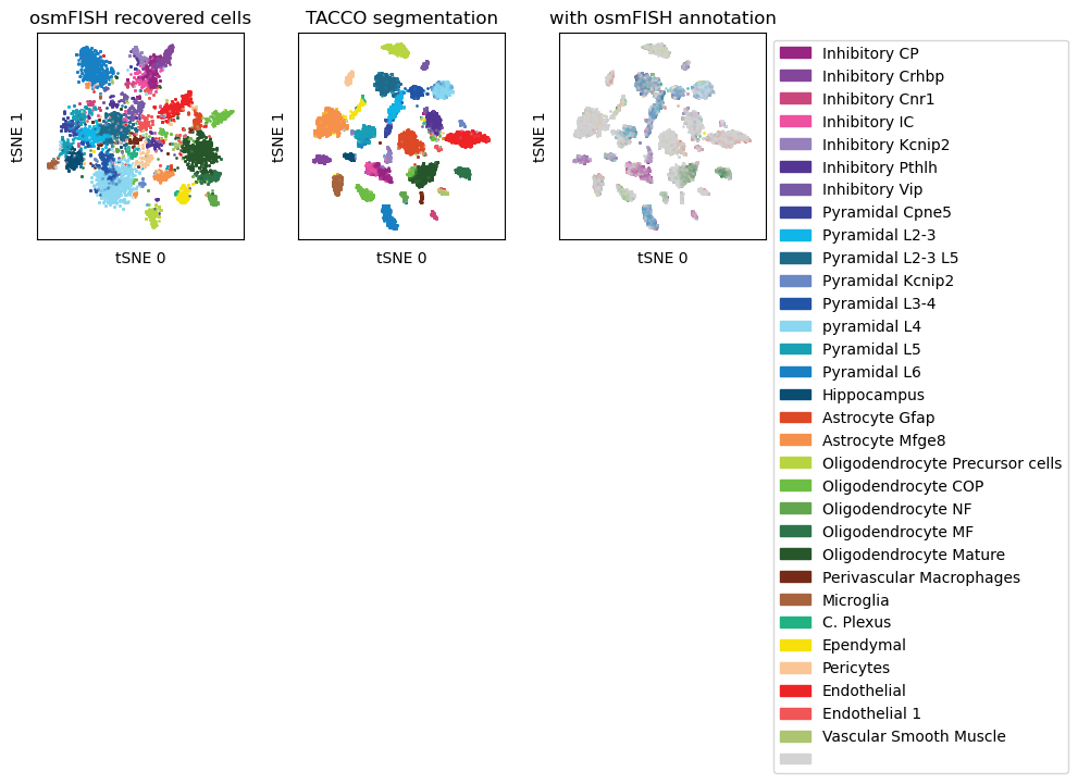
Compare the TACCO segmentation to the watershed segmentation results from (Codeluppi et al.)
[11]:
fig,axs = tc.pl.subplots(3, axsize=(1.9,1.9), x_padding=0.5)
tc.pl.scatter(norm_datas['reference'],'ClusterName', position_key='X_tsne', colors=color_dict, joint=True, noticks=True, margin=0.1, axes_labels=['tSNE 0','tSNE 1'], ax=axs[0,0], legend=False, );
tc.pl.scatter(norm_datas['TonT'],     'tacco',       position_key='X_tsne', colors=color_dict, joint=True, noticks=True, margin=0.1, axes_labels=['tSNE 0','tSNE 1'], ax=axs[0,1], legend=False, );
tc.pl.scatter(norm_datas['TonT'],     'ClusterName', position_key='X_tsne', colors=color_dict, joint=True, noticks=True, margin=0.1, axes_labels=['tSNE 0','tSNE 1'], ax=axs[0,2], legend=True, );
axs[0,0].set_title('osmFISH recovered cells')
axs[0,1].set_title('TACCO segmentation')
axs[0,2].set_title('with osmFISH annotation')
[11]:
Text(0.5, 1.0, 'with osmFISH annotation')
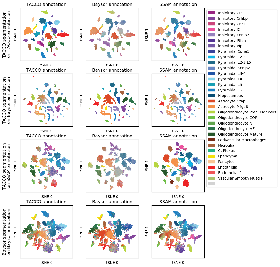
Cross-comparison of annotations of different methods with combinations of segmentation methods and annotations used in the segmentation
[12]:
fig,axs = tc.pl.subplots(len(method_keys),len(seg_props), axsize=(2.0,2.0), x_padding=0.5, y_padding=0.5)
for i_data,key in enumerate(seg_props.index):
    for j_method,method in enumerate(method_keys):
        tc.pl.scatter(norm_datas[key],method,    position_key='X_tsne', colors=color_dict, joint=True, noticks=True, margin=0.1, axes_labels=['tSNE 0','tSNE 1'], ax=axs[i_data,j_method], legend=((i_data==0) and (j_method==len(method_keys)-1)), );
        axs[i_data,j_method].set_title(f'{method_props.loc[method,"nice_name"]} annotation')
    axs[i_data,0].text(-0.25, 0.5, seg_props.loc[key,"nice_name"], fontsize='large', rotation=90, horizontalalignment='center', verticalalignment='center', transform=axs[i_data,0].transAxes)
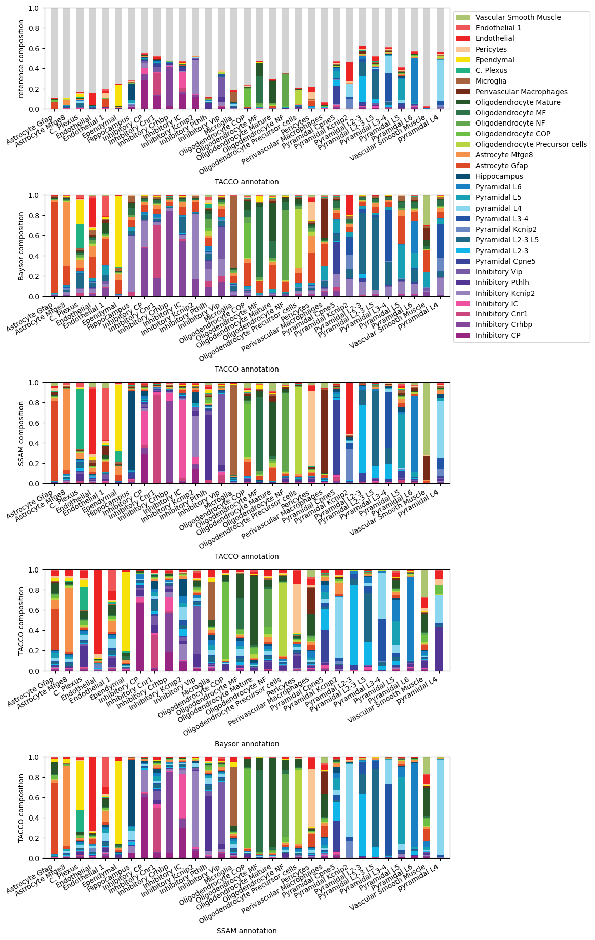
[13]:
fig,axs = tc.pl.subplots(1,5, axsize=(8,2), y_padding=1.7)
ax=axs[0,0]; tc.pl.compositions(seg_datas['TonT'], 'ClusterName', 'tacco',  colors=color_dict, reads=True, ax=ax);              ax.set_ylabel('reference composition'); ax.set_xlabel('TACCO annotation');
ax=axs[1,0]; tc.pl.compositions(seg_datas['TonT'], 'baysor',      'tacco',  colors=color_dict, reads=True, ax=ax,legend=False); ax.set_ylabel('Baysor composition');    ax.set_xlabel('TACCO annotation');
ax=axs[2,0]; tc.pl.compositions(seg_datas['TonT'], 'ssam',        'tacco',  colors=color_dict, reads=True, ax=ax,legend=False); ax.set_ylabel('SSAM composition');      ax.set_xlabel('TACCO annotation');
ax=axs[3,0]; tc.pl.compositions(seg_datas['TonB'], 'tacco',       'baysor', colors=color_dict, reads=True, ax=ax,legend=False); ax.set_ylabel('TACCO composition');     ax.set_xlabel('Baysor annotation');
ax=axs[4,0]; tc.pl.compositions(seg_datas['TonS'], 'tacco',       'ssam',   colors=color_dict, reads=True, ax=ax,legend=False); ax.set_ylabel('TACCO composition');     ax.set_xlabel('SSAM annotation');
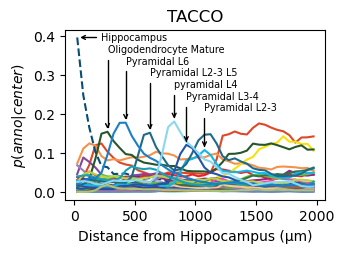
Find spatial layered structure using the TACCO segmented data
[14]:
analysis_key=f'tacco-tacco'
tc.tl.co_occurrence(seg_datas['TonT'], 'tacco', delta_distance=50, max_distance=2000, sparse=False, result_key=analysis_key);
fig = tc.pl.co_occurrence(seg_datas['TonT'], analysis_key, score_key='composition', colors=color_dict, wspace=0.3, show_only_center=['Hippocampus'], legend=False, axsize=(2.6,1.7), grid=False);
# annotate selected peaks in the data
ax = fig.get_axes()[0]
selection = pd.DataFrame({'anno':['Hippocampus','Oligodendrocyte Mature','Pyramidal L2-3','Pyramidal L2-3 L5','Pyramidal L3-4','pyramidal L4','Pyramidal L6']})
all_annotations = seg_datas['TonT'].uns[analysis_key]['annotation']
selection['anno_idx'] = selection['anno'].map(lambda x: np.argmax(all_annotations == x))
lines = ax.get_lines()
selection['y'] = selection['anno_idx'].map(lambda x: lines[x].get_ydata()[np.argmax(lines[x].get_ydata())])
selection['x'] = selection['anno_idx'].map(lambda x: lines[x].get_xdata()[np.argmax(lines[x].get_ydata())])
selection.sort_values('x', inplace=True)

for i,row in enumerate(selection.itertuples()):
    arrowprops = dict(arrowstyle="->",connectionstyle="arc", relpos=(0., 0.5))
    ax.annotate(row.anno,
            xy=(row.x, row.y), xycoords='data', ha="left", va="center", fontsize='x-small',
            xytext=(row.x + (200 if i==0 else 0), selection['y'].max()-0.21*i/len(selection)), textcoords='data',
            arrowprops=arrowprops,
            )

ax.set_title(f'TACCO')
ax.set_ylabel(f'$p(anno|center)$')
ax.set_xlabel(f'Distance from Hippocampus (µm)')
co_occurrence: The argument `distance_key` is `None`, meaning that the distance which is now calculated on the fly will not be saved. Providing a precalculated distance saves time in multiple calls to this function.
calculating distance for sample 1/1
[14]:
Text(0.5, 0, 'Distance from Hippocampus (µm)')
[15]:
reference.obs['x'] = reference.obs['X'] * reference.uns['um_per_pixel']
reference.obs['y'] = reference.obs['Y'] * reference.uns['um_per_pixel']
[16]:
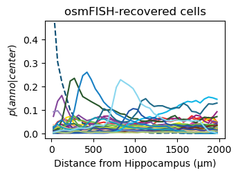
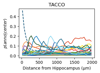
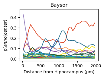
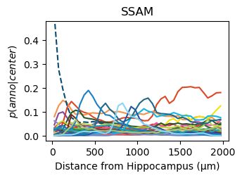
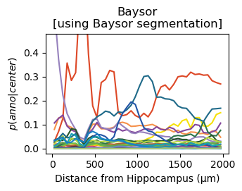
for method,seg,nice_ann in zip(ext_seg_props['ann_col'],ext_seg_props.index,ext_seg_props['nice_ann']):
    analysis_key=f'{method}-Hippocampus'
    filtered = seg_datas[seg][tc.sum(seg_datas[seg].X,axis=1) > segmented_min_counts].copy()
    tc.tl.co_occurrence(filtered, method, center_key='ClusterName', delta_distance=50, max_distance=2000, sparse=False, result_key=analysis_key);
    fig = tc.pl.co_occurrence(filtered, analysis_key, score_key='composition', colors=color_dict, wspace=0.3, show_only_center=['Hippocampus'], legend=False, axsize=(2.6,1.7), grid=False);
    fig.get_axes()[0].set_ylim([-0.02,0.48])
    fig.get_axes()[0].set_title(nice_ann)
    fig.get_axes()[0].set_ylabel(f'$p(anno|center)$')
    fig.get_axes()[0].set_xlabel(f'Distance from Hippocampus (µm)')
co_occurrence: The argument `distance_key` is `None`, meaning that the distance which is now calculated on the fly will not be saved. Providing a precalculated distance saves time in multiple calls to this function.
calculating distance for sample 1/1
co_occurrence: The argument `distance_key` is `None`, meaning that the distance which is now calculated on the fly will not be saved. Providing a precalculated distance saves time in multiple calls to this function.
calculating distance for sample 1/1
co_occurrence: The argument `distance_key` is `None`, meaning that the distance which is now calculated on the fly will not be saved. Providing a precalculated distance saves time in multiple calls to this function.
calculating distance for sample 1/1
co_occurrence: The argument `distance_key` is `None`, meaning that the distance which is now calculated on the fly will not be saved. Providing a precalculated distance saves time in multiple calls to this function.
calculating distance for sample 1/1
co_occurrence: The argument `distance_key` is `None`, meaning that the distance which is now calculated on the fly will not be saved. Providing a precalculated distance saves time in multiple calls to this function.
calculating distance for sample 1/1
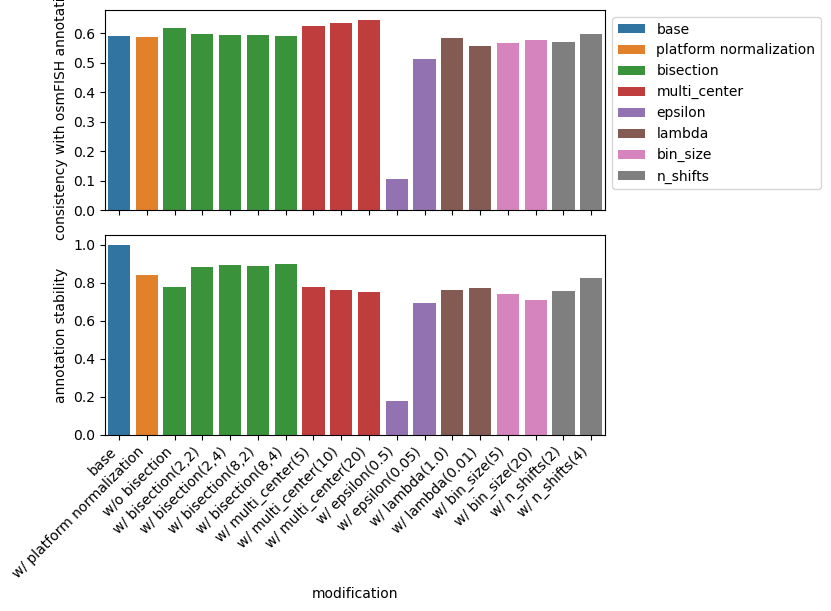
Get an impression of the stability of TACCO’s single molecule annotation wrt changes in its configuration
[17]:
mod_props = pd.DataFrame([
    [ 'tacco', 'base', 'base', 'base', ],
    [ 'tacco_pla0', 'pla0', 'w/ platform normalization', 'platform normalization', ],
    [ 'tacco_bisWO', 'bisWO', 'w/o bisection', 'bisection', ],
    [ 'tacco_bis22', 'bis22', 'w/ bisection(2,2)', 'bisection', ],
    [ 'tacco_bis24', 'bis24', 'w/ bisection(2,4)', 'bisection', ],
    [ 'tacco_bis82', 'bis82', 'w/ bisection(8,2)', 'bisection', ],
    [ 'tacco_bis84', 'bis84', 'w/ bisection(8,4)', 'bisection', ],
    [ 'tacco_mul5', 'mul5', 'w/ multi_center(5)', 'multi_center', ],
    [ 'tacco_mul10', 'mul10', 'w/ multi_center(10)', 'multi_center', ],
    [ 'tacco_mul20', 'mul20', 'w/ multi_center(20)', 'multi_center', ],
    [ 'tacco_eps05', 'eps05', 'w/ epsilon(0.5)', 'epsilon', ],
    [ 'tacco_eps005', 'eps005', 'w/ epsilon(0.05)', 'epsilon', ],
    [ 'tacco_lam1', 'lam1', 'w/ lambda(1.0)', 'lambda', ],
    [ 'tacco_lam001', 'lam001', 'w/ lambda(0.01)', 'lambda', ],
    [ 'tacco_bin5', 'bin5', 'w/ bin_size(5)', 'bin_size', ],
    [ 'tacco_bin20', 'bin20', 'w/ bin_size(20)', 'bin_size', ],
    [ 'tacco_nsh2', 'nsh2', 'w/ n_shifts(2)', 'n_shifts', ],
    [ 'tacco_nsh4', 'nsh4', 'w/ n_shifts(4)', 'n_shifts', ],
], columns=['key','mod','nice','group']).set_index('key')

comps = pd.DataFrame(index=mod_props.index)
for key in mod_props.index:
    comps[key] = [(rna_coords[key] == rna_coords[key2]).mean() for key2 in mod_props.index]

sub = rna_coords[rna_coords['ClusterName']!='']
accuracy = {key2: (sub[f'ClusterName'] == sub[key2]).mean() for key2 in mod_props.index}

plot_df = comps.iloc[:,[0]].copy().rename(columns={'tacco':'annotation stability'})
plot_df['group'] = plot_df.index.map(mod_props['group'])
plot_df['consistency with osmFISH annotation'] = plot_df.index.map(accuracy)
plot_df.index = comps.index.map(mod_props['nice'])
plot_df.index.name = 'modification'
plot_df = plot_df.reset_index()

fig,axs = tc.pl.subplots(1,2, axsize=(5,2), sharex=True, y_padding=0.25)
sns.barplot(data=plot_df, x='modification', y='consistency with osmFISH annotation', hue='group', dodge=False, ax=axs[0,0])
axs[0,0].set_xlabel(None);
axs[0,0].legend(bbox_to_anchor=(1, 1), loc='upper left')
sns.barplot(data=plot_df, x='modification', y='annotation stability', hue='group', dodge=False, ax=axs[1,0])
axs[1,0].set_xticklabels(axs[1,0].get_xticklabels(), rotation=45, ha='right', );
axs[1,0].get_legend().remove()